A meta analysis on effects of Parkinson’s Disease using Gemma.R
B. Ogan Mancarci
Michael Smith Laboratories, University of British Columbia, Vancouver, CanadaSource:
vignettes/metanalysis.Rmd
metanalysis.RmdGemma.R contains a large number of datasets representing a wide array of conditions. These datasets are manually annotated by our curators to facilitate discovery and categorization making it a useful tool for meta-analysis.
In this example we search Gemma for datasets comparing healthy controls and patients with Parkinson’s Disease. Our curators use ontology terms to annotate datasets when possible. This allows us to use the MONDO Disease Ontology term “MONDO:0005180” to search for datasets and samples annotated with the term to make sure we are accessing datasets relevant for our purposes with minimal effort.
Identifying what to search for
Gemma allows searching for datasets using plain text queries. However for a structured analysis, it is usually more helpful to use ontology terms to make sure we are getting the right datasets. To identify potentially useful ontology terms, we can use search_annotations
annots <- search_annotations("parkinson's")
annots %>% head %>% gemma_kable()| category.name | category.URI | value.name | value.URI |
|---|---|---|---|
| NA | NA | parkinson’s disease symptom… | http://www.ebi…/EFO_0600011 |
| NA | NA | secondary parkinson disease | http://www.ebi…/EFO_1001175 |
| NA | NA | wolff-parkinson-white syndrome | http://www.ebi…/EFO_1001450 |
| NA | NA | parkinson disease 6 | http://www.ebi…/EFO_0022988 |
| NA | NA | postencephalitic parkinson … | http://www.ebi…/EFO_1001402 |
| NA | NA | parkinson disease, dominant | http://www.ebi…/EFO_0022609 |
This will return matching ontology terms within every ontology loaded to Gemma. To identify which ones are actually used to annotate our datasets, you can do
annot_counts <- annots$value.URI %>% sapply(\(x){
    attributes(get_datasets(uris = x))$totalElements
})

annots$counts = annot_counts

annots %>% filter(counts>0) %>%
arrange(desc(counts)) %>% gemma_kable()| category.name | category.URI | value.name | value.URI | counts |
|---|---|---|---|---|
| NA | NA | parkinson disease | http://purl.obolibrary…/MONDO_0005180 | 215 |
| NA | NA | late-onset parkinson disease | http://purl.obolibrary…/MONDO_0008199 | 3 |
| NA | NA | autosomal dominant parkinso… | http://purl.obolibrary…/MONDO_0011764 | 2 |
| NA | NA | amyotrophic lateral scleros… | http://purl.obolibrary…/MONDO_0007104 | 2 |
| NA | NA | young-onset parkinson disease | http://purl.obolibrary…/MONDO_0017279 | 1 |
| NA | NA | autosomal dominant parkinso… | http://purl.obolibrary…/MONDO_0008200 | 1 |
| NA | NA | autosomal recessive juvenil… | http://purl.obolibrary…/MONDO_0010820 | 1 |
| NA | NA | x-linked dystonia-parkinsonism | http://purl.obolibrary…/MONDO_0010747 | 1 |
Querying datasets of interest
The get_datasets function can be used to find datasets
of interest, either using ontology terms or plain text. Since
Parkinson’s Disease has an unambiguous ontology term in the Disease
Ontology, we will be using it to avoid acquiring datasets that
tangentially mention the disease in their descriptions. Here we also
limit our results to only include human samples since we are not
interested in models from other species and samples that are explicitly
from the brain using the ontology term for brain. Here we will searching
within “allCharacteristics” however other filter properties are
available. You can use filter_properties to access all
available properties for anything filterable in Gemma.
Some noteable ones for our purposes would be “allCharacteristics”, which searches within every annotation on a dataset and its samples while we could have also used “experimentalDesign.experimentalFactors.factorValues.characteristics” to specifically look within experimental factors. Instead we will be showing how to limit for relevant contrasts in the next steps for this example.
filter_properties()$dataset %>% head %>% gemma_kable| properties | type | description |
|---|---|---|
| accession.accession | string | NA |
| accession.accessionVersion | string | NA |
| accession.externalDatabase…. | string | NA |
| accession.externalDatabase.id | integer | NA |
| accession.externalDatabase…. | string | NA |
| accession.externalDatabase…. | string | NA |
# getting all resulting datasets using limit and offset arguments
results <- get_datasets(filter = "allCharacteristics.valueUri = http://purl.obolibrary.org/obo/MONDO_0005180 and allCharacteristics.valueUri = http://purl.obolibrary.org/obo/UBERON_0000955",
                       taxa ='human') %>% get_all_pages()


results %>% select(experiment.shortName,experiment.name) %>% head
experiment.shortName
<char>
1: GSE7621
2: GSE7307
3: GSE8397
4: GSE20168
5: GSE20333
6: GSE20146
experiment.name
<char>
1: Expression data of substantia nigra from postmortem human brain of Parkinson's disease patients (PD)
2: Human body index - transcriptional profiling
3: Expression profiling of the Parkinsonian Brain
4: Transcriptional analysis of prefrontal area 9 in Parkinson's disease
5: Gene expression profiling of parkinsonian substantia nigra
6: Expression analysis of dissected GPi in Parkinson's diseaseFiltering the datasets for suitability
While we know that all the resulting datasets were annotated for the term for Parkinson’s Disease, we currently do not know how many of them are comparisons of healthy controls and patients with Parkinson’s Disease. We also do not know if the datasets have batch effects that may affect our findings.
For this example, we decided we should not include data sets that
have a batch confound (though that is up to the user). Gemma internally
handles batch correction if batch information is available for the
dataset. We will be looking at experiment.batchEffect
column. As explained in the get_datasets documentation,
this column will be set to -1 for datasets where batch confound is
detected, 0 for datasets without available batch information and to 1 if
the data is clear of batch confounds.
We now want to ensure that the differential expressions we analyze
compare control and Parkinson’s Disease patients. This information is
available via get_dataset_differential_expression_analyses
which returns the experimental groups for differential expression
analyses performed for the dataset. The columns we are primarily
interested in are baseline.factors which typically records
the control group of the differential expression analysis and
experimental.factors which typically records the test
case
experiment_contrasts <- results$experiment.shortName %>%
    lapply(function(x){
        out = get_dataset_differential_expression_analyses(x)
        }) %>% do.call(rbind,.)
The factor we are interested in is Parkinson’s Disease in
experimental.factorValue or “http://purl.obolibrary.org/obo/MONDO_0005180” in
experimental.factors’s value.URI. We also need
to make sure that the baseline that the sample is compared against is a
control experiment, samples annotated with “reference subject role” or
“http://purl.obolibrary.org/obo/OBI_0000220”
parkin_contrasts <- experiment_contrasts %>%
    filter(factor.category == 'disease') %>%
    filter(sapply(experimental.factors,function(x){
        "http://purl.obolibrary.org/obo/MONDO_0005180" %in% x$value.URI
        }) &
           sapply(baseline.factors,function(x){
               "http://purl.obolibrary.org/obo/OBI_0000220" %in% x$value.URI
               }))
Note that while this example attempts to show ways you can automate this process, you should take care to perform some manual examination of the data and determine how independent the contrasts you selected actually are. For instance in our selection, there are two contrasts from the same experiment where differential expression is performed on different brain regions.
[1] "873" "23781" result.ID contrast.ID experiment.ID factor.category
<int> <char> <int> <char>
1: 583617 17505 873 disease
2: 583618 17505 873 disease
3: 583619 17505 873 disease
4: 509632 200926 23781 disease
5: 509633 200926 23781 disease
factor.category.URI factor.ID baseline.factors
<char> <char> <list>
1: http://www.ebi.ac.uk/efo/EFO_0000408 2093 <data.table[1x13]>
2: http://www.ebi.ac.uk/efo/EFO_0000408 2093 <data.table[1x13]>
3: http://www.ebi.ac.uk/efo/EFO_0000408 2093 <data.table[1x13]>
4: http://www.ebi.ac.uk/efo/EFO_0000408 41659 <data.table[1x13]>
5: http://www.ebi.ac.uk/efo/EFO_0000408 41659 <data.table[1x13]>
experimental.factors isSubset subsetFactor probes.analyzed
<list> <lgcl> <list> <int>
1: <data.table[1x13]> TRUE <data.table[1x13]> 22282
2: <data.table[1x13]> TRUE <data.table[1x13]> 22282
3: <data.table[1x13]> TRUE <data.table[1x13]> 22283
4: <data.table[1x13]> TRUE <data.table[1x13]> 12040
5: <data.table[1x13]> TRUE <data.table[1x13]> 11708
genes.analyzed
<int>
1: 13327
2: 13327
3: 13327
4: 10588
5: 10298We should at least make sure that these two contrasts don’t share samples between them, one thing to check is the subsetFactor which might explain why these two separate contrasts exist
[[1]]
        category                         category.URI
          <char>                               <char>
1: organism part http://www.ebi.ac.uk/efo/EFO_0000635
                              value
                             <char>
1: substantia nigra pars reticulata
                                       value.URI predicate predicate.URI object
                                          <char>    <lgcl>        <lgcl> <lgcl>
1: http://purl.obolibrary.org/obo/UBERON_0001966        NA            NA     NA
   object.URI                          summary    ID factor.ID factor.category
       <lgcl>                           <char> <int>     <int>          <char>
1:         NA substantia nigra pars reticulata 17506      2094   organism part
                    factor.category.URI
                                 <char>
1: http://www.ebi.ac.uk/efo/EFO_0000635

[[2]]
        category                         category.URI
          <char>                               <char>
1: organism part http://www.ebi.ac.uk/efo/EFO_0000635
                            value                                     value.URI
                           <char>                                        <char>
1: substantia nigra pars compacta http://purl.obolibrary.org/obo/UBERON_0001965
   predicate predicate.URI object object.URI                        summary
      <lgcl>        <lgcl> <lgcl>     <lgcl>                         <char>
1:        NA            NA     NA         NA substantia nigra pars compacta
      ID factor.ID factor.category                  factor.category.URI
   <int>     <int>          <char>                               <char>
1: 17507      2094   organism part http://www.ebi.ac.uk/efo/EFO_0000635

[[3]]
        category                         category.URI                  value
          <char>                               <char>                 <char>
1: organism part http://www.ebi.ac.uk/efo/EFO_0000635 superior frontal gyrus
                                       value.URI predicate predicate.URI object
                                          <char>    <lgcl>        <lgcl> <lgcl>
1: http://purl.obolibrary.org/obo/UBERON_0002661        NA            NA     NA
   object.URI                summary    ID factor.ID factor.category
       <lgcl>                 <char> <int>     <int>          <char>
1:         NA superior frontal gyrus 17508      2094   organism part
                    factor.category.URI
                                 <char>
1: http://www.ebi.ac.uk/efo/EFO_0000635

[[4]]
    category                         category.URI                        value
      <char>                               <char>                       <char>
1: cell type http://www.ebi.ac.uk/efo/EFO_0000324 midbrain dopaminergic neuron
                                   value.URI    predicate
                                      <char>       <char>
1: http://purl.obolibrary.org/obo/CL_2000097 derives from
                               predicate.URI                 object
                                      <char>                 <char>
1: http://purl.obolibrary.org/obo/RO_0001000 ventral tegmental area
                                      object.URI
                                          <char>
1: http://purl.obolibrary.org/obo/UBERON_0002691
                                                            summary     ID
                                                             <char>  <int>
1: midbrain dopaminergic neuron derived from ventral tegmental area 200925
   factor.ID factor.category                  factor.category.URI
       <int>          <char>                               <char>
1:     41658   organism part http://www.ebi.ac.uk/efo/EFO_0000635

[[5]]
    category                         category.URI                        value
      <char>                               <char>                       <char>
1: cell type http://www.ebi.ac.uk/efo/EFO_0000324 midbrain dopaminergic neuron
                                   value.URI    predicate
                                      <char>       <char>
1: http://purl.obolibrary.org/obo/CL_2000097 derives from
                               predicate.URI                         object
                                      <char>                         <char>
1: http://purl.obolibrary.org/obo/RO_0001000 substantia nigra pars compacta
                                      object.URI
                                          <char>
1: http://purl.obolibrary.org/obo/UBERON_0001965
                                                                    summary
                                                                     <char>
1: midbrain dopaminergic neuron derived from substantia nigra pars compacta
       ID factor.ID factor.category                  factor.category.URI
    <int>     <int>          <char>                               <char>
1: 200924     41658   organism part http://www.ebi.ac.uk/efo/EFO_0000635
And we can see that these two contrasts are created to split the samples between different brain regions, therefore do not actually share samples between them.
In the next steps we will be downloading expression data in bulk. If you are here to just try the code out, you can speed the process a bit by limiting the number of experiments to deal with
# arbitrarily select a few datasets
# not executed in this example
parkin_contrasts <- parkin_contrasts[1:5,]
Now that we have our relevant contrasts, we can download them using
get_differential_expression_values. This function can be
used to download differential expression fold change and p values,
either using the experiment name/ids or more specifically using the
result.IDs
differentials <- parkin_contrasts$result.ID %>% lapply(function(x){
    # take the first and only element of the output. the function returns a list
    # because single experiments may have multiple resultSets. Here we use the
    # resultSet argument to directly access the results we need
    get_differential_expression_values(resultSets = x)[[1]]
})

# some datasets might not have all the advertised differential expression results
# calculated due to a variety of factors. here we remove the empty differentials
missing_contrasts <- differentials %>% sapply(nrow) %>% {.==0}
differentials <- differentials[!missing_contrasts]
parkin_contrasts <- parkin_contrasts[!missing_contrasts,]
Getting the p-values for the condition comparison
differentials is now a list of data frames containing
the differential expression information. To run a simple meta-analysis,
we need the p values for the genes from the relevant contrasts.
condition_diffs <- seq_along(differentials) %>% lapply(function(i){
    # iterate over the differentials
    diff = differentials[[i]]
    # get the contrast information about the differential
    contrast = parkin_contrasts[i,]
    p_vals = diff[[paste0('contrast_',contrast$contrast.ID,"_pvalue")]]
    log2fc = diff[[paste0('contrast_',contrast$contrast.ID,"_log2fc")]]
    genes = diff$GeneSymbol

    data.frame(genes,p_vals,log2fc)
})

# we can use result.IDs and contrast.IDs to uniquely name this.
# we add the experiment.id for readability
names(condition_diffs) = paste0(parkin_contrasts$experiment.ID,'.',
                                parkin_contrasts$result.ID,'.',
                                parkin_contrasts$contrast.ID)

condition_diffs[[1]] %>% head
genes p_vals log2fc
1 XIST 3.570e-02 -0.3767
2 DDX3Y 1.000e-04 0.6292
3 XIST 2.100e-02 0.2353
4 SELE 1.519e-13 -3.9249
5 XIST 8.200e-03 0.2929
6 XIST 4.010e-01 -0.1258Combining the acquired p values
Now that we have acquired the values we need for a meta-analysis from Gemma, we can proceed with any methodology we deem suitable for our analysis.
In this example we will use a very simple approach, Fisher’s combined
p-value test. This is implemented in the fisher
function from poolr package. Fisher’s method has the
advantage that it operates on the p-values, which are in the processed
differential expression results in Gemma. It has some disadvantages like
ignoring the direction of the expression change (Gemma’s p-values are
two-tailed) and is very sensitive to a single ‘outlier’ p-value, but for
this demonstration we’ll go with it.
The first step is to identify which genes are available in our results:
all_genes <- condition_diffs %>% lapply(function(x){
    x$genes %>% unique
}) %>% unlist %>% table

# we will remove any gene that doesn't appear in all of the results
# while this criteria is too strict, it does help this example to run
# considerably faster
all_genes <- all_genes[all_genes==max(all_genes)]
all_genes <- names(all_genes)

# remove any probesets matching multiple genes. gemma separates these by using "|"
all_genes <- all_genes[!grepl("|",all_genes,fixed = TRUE)]

# remove the "". This comes from probesets not aligned to any genes
all_genes <- all_genes[all_genes != ""]
all_genes %>% head
[1] "A2M" "AAAS" "AACS" "AAGAB" "AAK1" "AAMP" Now we can run the test on every gene, followed by a multiple testing correction.
fisher_results <- all_genes %>% lapply(function(x){
    p_vals <- condition_diffs %>% sapply(function(y){
        # we will resolve multiple probesets by taking the minimum p value for
        # this example
        out = y[y$genes == x,]$p_vals
        if(length(out) == 0 ||all(is.na(out))){
            return(NA)
        } else{
            return(min(out))
        }
    })

    fold_changes <- condition_diffs %>% sapply(function(y){
        pv = y[y$genes == x,]$p_vals
        if(length(pv) == 0 ||all(is.na(pv))){
            return(NA)
        } else{
            return(y[y$genes == x,]$log2fc[which.min(pv)])
        }
    })

    median_fc = fold_changes %>% na.omit() %>% median
    names(median_fc) = 'Median FC'

    combined = p_vals %>% na.omit() %>% fisher() %>% {.$p}
    names(combined) = 'Combined'
    c(p_vals,combined,median_fc)
}) %>% do.call(rbind,.)
fisher_results <- as.data.frame(fisher_results)
rownames(fisher_results) = all_genes

fisher_results[,'Adjusted'] <- p.adjust(fisher_results[,'Combined'],
                                        method = 'fdr')

fisher_results %>%
    arrange(Adjusted) %>%
    select(Combined,Adjusted,`Median FC`) %>%
    head
We end up with quite a few differentially expressed genes in the meta-analysis (Fisher’s method is very sensitive)
sum(fisher_results$Adjusted<0.05) # FDR<0.05[1] 5346
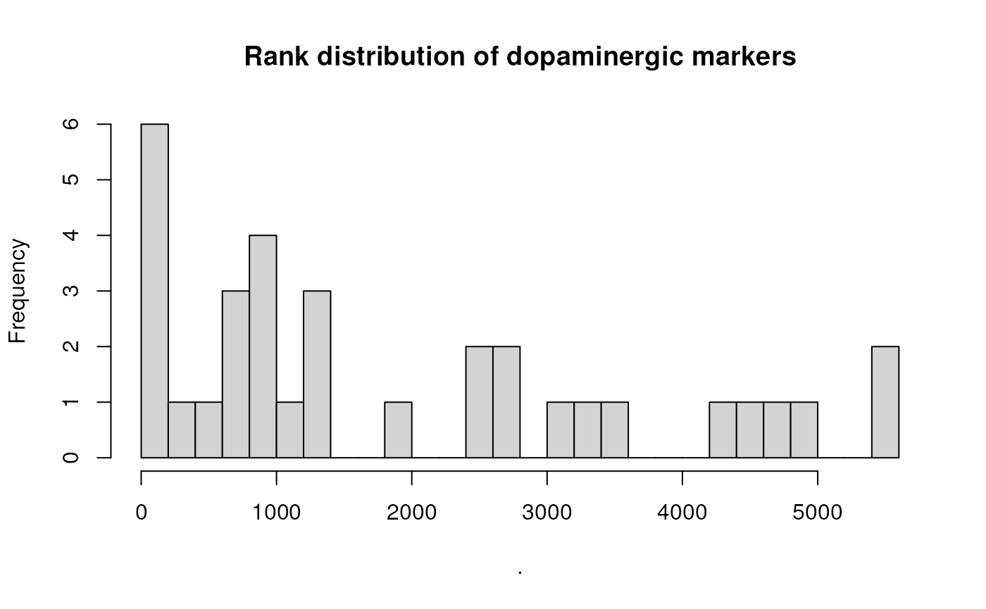
nrow(fisher_results) # number of all genes[1] 6252Next we look at markers of dopaminergic cell types and how they rank compared to other genes. Parkinson’s Disease is a neurodegenerative disorder, leading to death of dopaminergic cells. We should expect them to show up in our results.
# markers are taken from https://www.eneuro.org/content/4/6/ENEURO.0212-17.2017
dopa_markers <-  c("ADCYAP1", "ATP2B2", "CACNA2D2",
"CADPS2", "CALB2", "CD200", "CDK5R2", "CELF4", "CHGA", "CHGB",
"CHRNA6", "CLSTN2", "CNTNAP2", "CPLX1", "CYB561", "DLK1", "DPP6",
"ELAVL2", "ENO2", "GABRG2", "GRB10", "GRIA3", "KCNAB2", "KLHL1",
"LIN7B", "MAPK8IP2", "NAPB", "NR4A2", "NRIP3", "HMP19", "NTNG1",
"PCBP3", "PCSK1", "PRKCG", "RESP18", "RET", "RGS8", "RNF157",
"SCG2", "SCN1A", "SLC12A5", "SLC4A10", "SLC6A17", "SLC6A3", "SMS",
"SNCG", "SPINT2", "SPOCK1", "SYP", "SYT4", "TACR3", "TENM1",
"TH", "USP29")

fisher_results %>%
    arrange(Combined) %>%
    rownames %>%
    {.%in% dopa_markers} %>%
    which %>%
    hist(breaks=20, main = 'Rank distribution of dopaminergic markers')
In agreement with our hypothesis, we can see that the dopaminergic markers tend to have high ranks in our results.
Acquiring the expression data for a top gene
Now that we have our results, we can take a look at how the
expression of one of our top genes in these experiments. To do this we
will use the get_dataset_expression_for_genes function to
get the expression data. Once we get the expression data for our genes
of interest, we will use the get_dataset_samples function
to identify which samples belongs to which experimental group.
Note: as of this writing (early 2023), the Gemma.R methods used in this section are not yet released in Bioconductor; install via devtools to try it out.
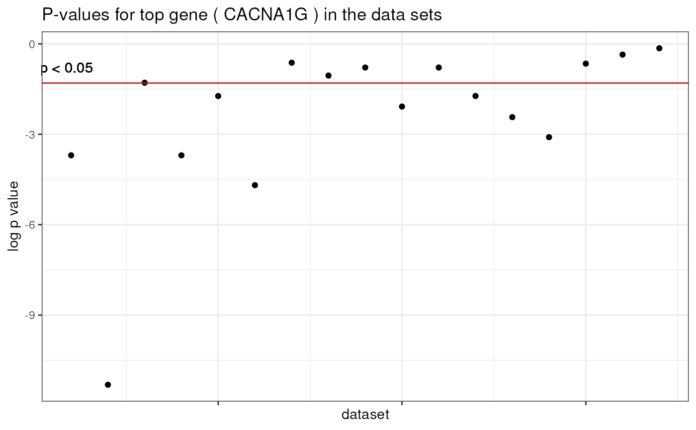
For starters, lets look at our top pick and the its p values in the individual datasets, on a log scale:
# the top gene from our results
gene <- fisher_results %>% arrange(Adjusted) %>% .[1,] %>% rownames

p_values <- fisher_results %>%
    arrange(Adjusted) %>%
    .[1,] %>%
    select(-Combined,-`Median FC`,-Adjusted) %>%
    unlist %>%
    na.omit()

#sum(p_values<0.05)
#length(p_values)

# p values of the result in individual studies
p_values %>% log10() %>%
    data.frame(`log p value` = .,dataset = 1:length(.),check.names = FALSE) %>%
    ggplot(aes(y = `log p value`,x = dataset)) +
    geom_point() +
    geom_hline(yintercept = log10(0.05),color = 'firebrick') +
    geom_text(y = log10(0.05), x = 0, label = 'p < 0.05',vjust =-1,hjust = -0.1) +
    theme_bw() + ggtitle(paste("P-values for top gene (", gene, ") in the data sets")) +
    theme(axis.text.x = element_blank())
This shows that the gene is nominally significant in some but not all of
the data sets.
To examine this further, our next step is to acquire gene expression
data from the relevant datasets using get_dataset_object.
We will use both dataset ids and resultSet ids when using this function
since some of the returned analysis are only performed on a subset of
the data. Providing resultSet ids allows us to harmonize the
differential expression results with expression data by returning the
relevant subset.
# we need the NCBI id of the gene in question, lets get that from the original
# results
NCBIid <- differentials[[1]] %>% filter(GeneSymbol == gene) %>% .$NCBIid %>% unique
#NCBIid


expression_frame <- get_dataset_object(datasets = parkin_contrasts$experiment.ID,
                                       resultSets = parkin_contrasts$result.ID,
                                       contrasts = parkin_contrasts$contrast.ID,
                                       genes = NCBIid,type = 'tidy',consolidate = 'pickvar')

# get the contrast names for significance markers
signif_contrasts <- which(p_values < 0.05) %>% names
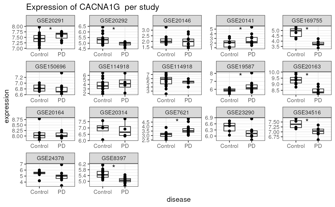
Finally, we’ll make a plot showing the expression of the gene of interest in all the data sets. This helps us see the extent to which there is evidence of consistent differential expression.
expression_frame <- expression_frame %>%
    filter(!is.na(expression)) %>%
    # add a column to represent the contrast
    dplyr::mutate(contrasts = paste0(experiment.ID,'.',
                                    result.ID,'.',
                                    contrast.ID)) %>%
    # simplify the labels
    dplyr::mutate(disease = ifelse(disease == 'reference subject role','Control','PD'))

# for adding human readable labels on the plot
labeller <- function(x){
    x %>% mutate(contrasts = contrasts %>%
                     strsplit('.',fixed = TRUE) %>%
                     purrr::map_chr(1) %>%
                     {expression_frame$experiment.shortName[match(.,expression_frame$experiment.ID)]})
}

# pass it all to ggplot
expression_frame %>%
    ggplot(aes(x = disease,y = expression)) +
    facet_wrap(~contrasts,scales = 'free',labeller = labeller) +
    theme_bw() +
    geom_boxplot(width = 0.5) +
    geom_point() + ggtitle(paste("Expression of", gene, " per study")) +
    geom_text(data = data.frame(contrasts = signif_contrasts,
                             expression_frame %>%
                             group_by(contrasts) %>%
                             summarise(expression = max(expression)) %>%
                             .[match(signif_contrasts,.$contrasts),]),
              x = 1.5, label = '*',size=5,vjust= 1)
Session info
R version 4.5.3 (2026-03-11)
Platform: x86_64-pc-linux-gnu
Running under: Ubuntu 24.04.4 LTS

Matrix products: default
BLAS:   /usr/lib/x86_64-linux-gnu/openblas-pthread/libblas.so.3
LAPACK: /usr/lib/x86_64-linux-gnu/openblas-pthread/libopenblasp-r0.3.26.so;  LAPACK version 3.12.0

locale:
 [1] LC_CTYPE=C.UTF-8       LC_NUMERIC=C           LC_TIME=C.UTF-8
 [4] LC_COLLATE=C.UTF-8     LC_MONETARY=C.UTF-8    LC_MESSAGES=C.UTF-8
 [7] LC_PAPER=C.UTF-8       LC_NAME=C              LC_ADDRESS=C
[10] LC_TELEPHONE=C         LC_MEASUREMENT=C.UTF-8 LC_IDENTIFICATION=C

time zone: UTC
tzcode source: system (glibc)

attached base packages:
[1] parallel  stats     graphics  grDevices utils     datasets  methods
[8] base

other attached packages:
[1] stringr_1.6.0    ggplot2_4.0.2    poolr_1.2-0      dplyr_1.2.0
[5] gemma.R_3.7.2    BiocStyle_2.38.0

loaded via a namespace (and not attached):
 [1] tidyr_1.3.2         sass_0.4.10         generics_0.1.4
 [4] xml2_1.5.2          stringi_1.8.7       digest_0.6.39
 [7] magrittr_2.0.4      timechange_0.4.0    evaluate_1.0.5
[10] grid_4.5.3          RColorBrewer_1.1-3  bookdown_0.46
[13] fastmap_1.2.0       jsonlite_2.0.0      BiocManager_1.30.27
[16] httr_1.4.8          purrr_1.2.1         viridisLite_0.4.3
[19] scales_1.4.0        textshaping_1.0.5   jquerylib_0.1.4
[22] cli_3.6.5           rlang_1.1.7         bit64_4.6.0-1
[25] withr_3.0.2         cachem_1.1.0        yaml_2.3.12
[28] otel_0.2.0          tools_4.5.3         mathjaxr_2.0-0
[31] kableExtra_1.4.0    assertthat_0.2.1    curl_7.0.0
[34] vctrs_0.7.2         R6_2.6.1            lubridate_1.9.5
[37] lifecycle_1.0.5     fs_2.0.1            htmlwidgets_1.6.4
[40] bit_4.6.0           ragg_1.5.2          pkgconfig_2.0.3
[43] desc_1.4.3          pkgdown_2.2.0       pillar_1.11.1
[46] bslib_0.10.0        gtable_0.3.6        data.table_1.18.2.1
[49] glue_1.8.0          systemfonts_1.3.2   xfun_0.57
[52] tibble_3.3.1        tidyselect_1.2.1    rstudioapi_0.18.0
[55] knitr_1.51          farver_2.1.2        htmltools_0.5.9
[58] labeling_0.4.3      svglite_2.2.2       rmarkdown_2.31
[61] compiler_4.5.3      S7_0.2.1