Accessing curated gene expression data with GemmaPy
About Gemma
Gemma is a web site, database and a set of tools for the meta-analysis, re-use and sharing of genomics data, currently primarily targeted at the analysis of gene expression profiles. Gemma contains data from thousands of public studies, referencing thousands of published papers. Every dataset in Gemma has passed a rigorous curation process that re-annotates the expression platform at the sequence level, which allows for more consistent cross-platform comparisons and meta-analyses.
For detailed information on the curation process, read this page or the latest publication.
Installation instructions
The package requires Python3.6+.
Install it from a local copy
git clone git@github.com:PavlidisLab/gemmapy.git
cd gemmapy
pip install .
Install it from PyPI
pip install gemmapy
Additional packages
For the purpose of making plots in this tutorial the following packages should be installed
and imported: matplotlib, plotnine, pandas, seaborn, statsmodels.
Searching for datasets of interest in Gemma
Using the get_datasets() function, datasets fitting various criteria can be accessed.
>>> import gemmapy
>>> api = gemmapy.GemmaPy()
>>> # accessing all mouse and human datasets
>>> api.get_datasets(taxa = ['mouse','human']).head()
  experiment_short_name  ... taxon_database_ID
0               GSE2018  ...                87
1               GSE4523  ...                81
2               GSE4036  ...                87
3               GSE4034  ...                81
4               GSE2866  ...                81
[5 rows x 23 columns]
>>> # accessing human datasets with the word "bipolar"
>>> api.get_datasets(query = 'bipolar', taxa = ['human']).head()
  experiment_short_name  ... taxon_database_ID
0             GSE157509  ...                87
1              GSE66196  ...                87
2             GSE210064  ...                87
3              GSE23848  ...                87
4    McLean Hippocampus  ...                87
[5 rows x 23 columns]
>>> # accessing human datasets that were annotated with the ontology term for
>>> # the bipolar disorder. use search_annotations function to search for available
>>> # annotation terms
>>> api.get_datasets(taxa = ['human'],
...    uris = ['http://purl.obolibrary.org/obo/MONDO_0004985']).head()
  experiment_short_name  ... taxon_database_ID
0               GSE5389  ...                87
1               GSE5388  ...                87
2               GSE7036  ...                87
3    McLean Hippocampus  ...                87
4            McLean_PFC  ...                87
[5 rows x 23 columns]
get_dataset function also includes a filter parameter that allows filtering for
datasets with specific properties in a more structured manner. A list of the
available properties can be accessed using filter_properties().
>>> api.filter_properties()['dataset'].head()
                                     name     type description
0                     accession.accession   string         NaN
1              accession.accessionVersion   string         NaN
2       accession.externalDatabase.ftpUri   string         NaN
3           accession.externalDatabase.id  integer         NaN
4  accession.externalDatabase.lastUpdated   string         NaN
These properties can be used together to fine tune your results
>>> # access human datasets that has bipolar disorder as an experimental factor
>>> api.get_datasets(taxa = ["human"],
...    filter = "experimentalDesign.experimentalFactors.factorValues.characteristics.valueUri = http://purl.obolibrary.org/obo/MONDO_0004985").head()
  experiment_short_name  ... taxon_database_ID
0               GSE5389  ...                87
1               GSE5388  ...                87
2               GSE7036  ...                87
3            McLean_PFC  ...                87
4      stanley_feinberg  ...                87
[5 rows x 23 columns]
>>> # all datasets with more than 4 samples annotated for any disease
>>> api.get_datasets(filter = "bioAssayCount > 4 and allCharacteristics.category = disease").head()
  experiment_short_name  ... taxon_database_ID
0               GSE2018  ...                87
1               GSE4036  ...                87
2               GSE2866  ...                81
3               GSE2426  ...                81
4               GSE2867  ...                81
[5 rows x 23 columns]
>>> # all datasets with ontology terms for Alzheimer's disease and Parkinson's disease
>>> # this is equivalent to using the uris parameter
>>> api.get_datasets(filter = 'allCharacteristics.valueUri in (http://purl.obolibrary.org/obo/MONDO_0004975,http://purl.obolibrary.org/obo/MONDO_0005180)').head()
  experiment_short_name  ... taxon_database_ID
0               GSE1837  ...                86
1                 GSE30  ...                81
2               GSE4788  ...                81
3               GSE1157  ...                86
4               GSE1555  ...                81
[5 rows x 23 columns]
Note that a single call of these functions will only return 20 results by default
and a 100 results maximum, controlled by the limit argument. In order to get all
available results, use get_all_pages()
>>> api.get_all_pages(api.get_datasets,taxa = ['human'])
     experiment_short_name  ... taxon_database_ID
0                  GSE2018  ...                87
1                  GSE4036  ...                87
2                  GSE3489  ...                87
3                  GSE1923  ...                87
4                   GSE361  ...                87
                   ...  ...               ...
7697              GSE72747  ...                87
7698                GSE976  ...                87
7699              GSE78083  ...                87
7700            GSE11142.2  ...                87
7701             GSE2489.2  ...                87
[7702 rows x 23 columns]
See Larger queries section for more details. To keep this vignette simpler we will keep using the first 20 results returned by default in examples below.
Dataset information provided by get_datasets also includes some quality information that can be used to determine the suitability of any given experiment. For instance experiment.batchEffect column will be set to -1 if Gemma’s preprocessing has detected batch effects that were unable to be resolved by batch correction. More information about these and other fields can be found at the function documentation.
>>> df = api.get_datasets(taxa = ['human'],filter = 'bioAssayCount > 4')
>>> df.loc[df.experiment_batch_effect != -1].head()
Gemma uses multiple ontologies when annotating datasets and using the term URIs
instead of free text to search can lead to more specific results.
search_annotations() function allows searching for
annotation terms that might be relevant to your query.
>>> api.search_annotations(['bipolar']).head()
   category_name  ...                                     value_URI
0            NaN  ...          http://www.ebi.ac.uk/efo/EFO_0009963
1            NaN  ...          http://www.ebi.ac.uk/efo/EFO_0009964
2            NaN  ...  http://purl.obolibrary.org/obo/MONDO_0004985
3            NaN  ...     http://purl.obolibrary.org/obo/HP_0007302
4            NaN  ...    http://purl.obolibrary.org/obo/NBO_0000258
[5 rows x 4 columns]
Downloading expression data
Upon identifying datasets of interest, more information about specific ones can be requested. In this example we will be using GSE46416 which includes samples taken from healthy donors along with manic/euthymic phase bipolar disorder patients.
The data associated with specific experiments can be accessed by using
get_datasets_by_ids().
>>> data = api.get_datasets_by_ids(['GSE46416'])
>>> print(data)
  experiment_short_name  ... taxon_database_ID
0              GSE46416  ...                87
[1 rows x 23 columns]
To access the expression data in a convenient form, you can use
get_dataset_object(). It is a high-level wrapper
that combines various endpoint calls to return anndata (Annotated Data) objects or dictionaries.
These include the expression matrix along with the experimental design, and
ensure the sample names match between both when transforming/subsetting data.
>>> adata = api.get_dataset_object(["GSE46416"])['8997']  # keys of the output uses Gemma IDs
>>> print(adata)
AnnData object with n_obs × n_vars = 18758 × 32
    obs: 'GeneSymbol', 'NCBIid'
    var: 'factor_values', 'disease', 'block'
    uns: 'title', 'abstract', 'url', 'database', 'accesion', 'GemmaQualityScore', 'GemmaSuitabilityScore', 'taxon'
To show how subsetting works, we’ll keep the “manic phase” data and the
reference_subject_roles, which refers to the control samples in Gemma
datasets.
>>> # Check the levels of the disease factor
>>> adata.var['disease'].unique()
array(['bipolar disorder has_modifier euthymic phase',
       'reference subject role',
       'bipolar disorder has_modifier manic phase'], dtype=object)
>>> # Subset patients during manic phase and controls
>>> manic=adata[:,(adata.var['disease'] == 'reference subject role') |
...               (adata.var['disease'] == 'bipolar disorder has_modifier manic phase')].copy()
>>> manic
AnnData object with n_obs × n_vars = 18758 × 21
    obs: 'GeneSymbol', 'NCBIid'
    var: 'factor_values', 'disease', 'block'
    uns: 'title', 'abstract', 'url', 'database', 'accesion', 'GemmaQualityScore', 'GemmaSuitabilityScore', 'taxon'
>>> manic.var.head()
                                                                              factor_values  ...              block
Control, 15                                 category  ...                   factor_categ...  ...  Batch_02_26/11/09
Control, 8                                  category  ...                   factor_categ...  ...  Batch_01_25/11/09
Bipolar disorder patient manic phase, 21    category  ...                   factor_categ...  ...  Batch_03_27/11/09
Bipolar disorder patient manic phase, 18    category  ...                   factor_categ...  ...  Batch_02_26/11/09
Bipolar disorder patient manic phase, 29    category  ...                   factor_categ...  ...  Batch_03_27/11/09
[5 rows x 3 columns]
Let’s take a look at sample to sample correlation in our subset.
>>> # get expression data frame
>>> import pandas as pd
>>> import seaborn as sns
>>> df = pd.DataFrame(manic.X)
>>> df.columns = manic.var.index
>>> corrs = df.corr()
>>> plt = sns.clustermap(corrs)
>>> plt.savefig('ded.png')
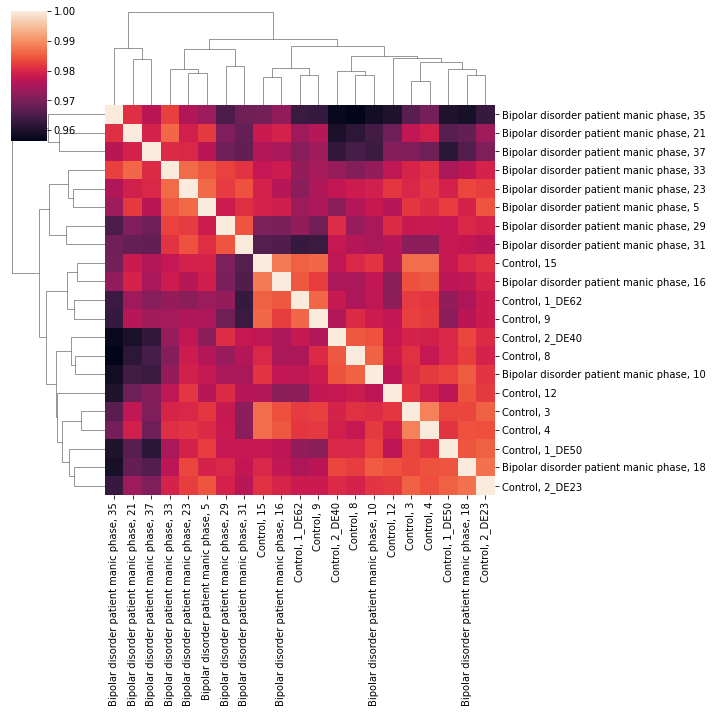
Sample to sample correlations of bipolar patients during manic phase and controls.
You can also use get_dataset_processed_expression() to only get the expression
matrix, and get_dataset_samples() to get the metadata
information. The output of this function includes some additional details about
a sample such as the original accession ID or whether or not it was determined
to be an outlier but it can be simplified to match the design table included in
the output of get_dataset_object by using make_design() on the output.
>>> api.make_design(api.get_dataset_samples('GSE46416')).drop(columns="factor_values").head()
                                                                                  disease              block
sample_name
Bipolar disorder patient euthymic phase, 17  bipolar disorder has_modifier euthymic phase  Batch_02_26/11/09
Bipolar disorder patient euthymic phase, 34  bipolar disorder has_modifier euthymic phase  Batch_04_02/12/09
Control, 15                                                        reference subject role  Batch_02_26/11/09
Bipolar disorder patient euthymic phase, 32  bipolar disorder has_modifier euthymic phase  Batch_04_02/12/09
Control, 8                                                         reference subject role  Batch_01_25/11/09
Platform Annotations
Expression data in Gemma comes with annotations for the gene each
expression profile corresponds to. Using the
get_platform_annotations() function, these
annotations can be retrieved independently of the expression data,
along with additional annotations such as Gene Ontology terms.
Examples:
>>> api.get_platform_annotations('GPL96').head()
     ProbeName    GeneSymbols  ...       GemmaIDs     NCBIids
0  211750_x_at  TUBA1C|TUBA1A  ...  360802|172797  84790|7846
1    216678_at            NaN  ...            NaN         NaN
2    216345_at         ZSWIM8  ...         235733       23053
3    207273_at            NaN  ...            NaN         NaN
4  216025_x_at         CYP2C9  ...          32964        1559
[5 rows x 6 columns]
>>> api.get_platform_annotations('Generic_human_ncbiIds').head()
>>> with pandas.option_context('display.max_rows', None, 'display.max_columns', None): print(api_response[:6])
   ElementName   GeneSymbols  ...    GemmaIDs      NCBIids
0        55236          UBA6  ...    295849.0      55236.0
1        79664          ICE2  ...    336840.0      79664.0
2    100126270      FMR1-AS1  ...   3157248.0  100126270.0
3    105373684     LINC01818  ...   9235895.0  105373684.0
4    124900245  LOC124900245  ...  10578422.0  124900245.0
[5 rows x 6 columns]
If you are interested in a particular gene, you can see which
platforms include it using
get_gene_probes(). Note that functions to
search gene work best with unambigious identifiers rather than symbols.
>>> # lists genes in gemma matching the symbol or identifier
>>> api.get_genes(['Eno2'])
  gene_symbol        gene_ensembl  ...  taxon_database_name taxon_database_ID
0        ENO2     ENSG00000111674  ...                 hg38                87
1        Eno2  ENSMUSG00000004267  ...                 mm10                81
2        Eno2  ENSRNOG00000013141  ...                  rn6                86
[3 rows x 12 columns]
>>> # ncbi id for human ENO2
>>> api.get_gene_probes("ENSG00000111674").head()
  element_name  ... taxon_database_ID
0    201313_at  ...                87
1    201313_at  ...                87
2     40193_at  ...                87
3         1639  ...                87
4         6621  ...                87
[5 rows x 14 columns]
Differential expression analyses
Gemma contains precomputed differential expression analyses for most
of its datasets. Analyses can involve more than one factor, such as
“sex” as well as “disease”. Some datasets contain more than one
analysis to account for different factors and their interactions. The
results are stored as resultSets, each corresponding to one factor (or
their interaction). You can access them using
get_differential_expression_values(). From here on, we can
explore and visualize the data to find the most
differentially-expressed genes.
Note that get_differential_expression_values() can
return multiple differentials per study if a study has multiple factors to contrast.
Since GSE46416 only has one extracting the first element of the returned list is all we need.
>>> dif_exp = api.get_differential_expression_values('GSE46416')
>>> dif_exp[list(dif_exp.keys())[0]]
{550248:          Probe     NCBIid  ... contrast_113005_tstat contrast_113005_pvalue
 0      2982730       4018  ...               -0.3622                 0.7196
 1      2787851     166752  ...                0.7495                 0.4590
 2      2477558        NaN  ...                1.2604                 0.2166
 3      2910917        NaN  ...                0.9032                 0.3731
 4      3983537     140886  ...                1.7656                 0.0869
       ...        ...  ...                   ...                    ...
 21956  3301011      64318  ...               -1.6208                 0.1148
 21957  2461654  100130249  ...               -0.2045                 0.8393
 21958  2360346       1141  ...                3.1278                 0.0037
 21959  2391172       7293  ...                1.7369                 0.0920
 21960  2525718        NaN  ...               -0.7101                 0.4827
 [21961 rows x 13 columns]}
By default the columns names of the output correspond to contrast IDs. To see
what conditions these IDs correspond to we can either use
get_dataset_differential_expression_analyses() to
get the metadata about differentials of a given dataset, or
readable_contrasts argument of
get_differential_expression_values() to True.
The former approach is usually better for a large scale systematic analysis
while the latter is easier to read in an interactive session.
get_dataset_differential_expression_analyses()
function returns metadata about the differentials.
>>> contrasts = api.get_dataset_differential_expression_analyses("GSE46416")
>>> contrasts
   result_ID contrast_ID  ...  probes_analyzed genes_analyzed
0     550248      113004  ...            21961          18959
1     550248      113005  ...            21961          18959
[2 rows x 12 columns]
contrast_ID column corresponds to the column names in the output of
get_differential_expression_values() while result_ID
corresponds to the name of the differential in the output object. Using them
together will let one to access differentially expressed gene counts for each
condition contrast
>>> import statsmodels.stats.multitest as multi
>>> dif_exp_genes = [
...    sum(multi.multipletests(
...        dif_exp[contrasts.loc[i,].result_ID][
...            "contrast_" + contrasts.loc[i,].contrast_ID + "_pvalue"
...            ],
...        alpha = 0.05, method = "fdr_bh")[0]) for i in range(contrasts.shape[0])]
>>> contrasts.assign(n_diff= dif_exp_genes)
>>> contrasts
   result_ID contrast_ID  ...  probes_analyzed genes_analyzed
0     550248      113004  ...            21961          18959
1     550248      113005  ...            21961          18959
[2 rows x 12 columns]
>>> # baseline factors of the contrasts
>>> [x.summary for x in contrasts.baseline_factors]
[0    reference subject role
 Name: summary, dtype: object,
 0    reference subject role
 Name: summary, dtype: object]
>>> # experimental factors of the contrasts
>>> [x.summary for x in contrasts.experimental_factors]
[0    bipolar disorder has_modifier manic phase
 Name: summary, dtype: object,
 0    bipolar disorder has_modifier euthymic phase
 Name: summary, dtype: object]
Alternatively we, since we are only looking at one dataset and one contrast manually, we can simply use readable_contrasts.
>>> de = api.get_differential_expression_values('GSE46416',readable_contrasts = True)
>>> de = de[list(de.keys())[0]]
>>> print(de)
         Probe  ... contrast_bipolar disorder has_modifier euthymic phase_pvalue
0      2982730  ...                                             0.7196
1      2787851  ...                                             0.4590
2      2477558  ...                                             0.2166
3      2910917  ...                                             0.3731
4      3983537  ...                                             0.0869
       ...  ...                                                ...
21956  3301011  ...                                             0.1148
21957  2461654  ...                                             0.8393
21958  2360346  ...                                             0.0037
21959  2391172  ...                                             0.0920
21960  2525718  ...                                             0.4827
[21961 rows x 13 columns]
>>> # Classify probes for plotting
>>> de['diffexpr'] = 'No'   # add extra column
>>> de.loc[(de['contrast_bipolar disorder has_modifier manic phase_logFoldChange'] > 1.0) &
...        (de['contrast_bipolar disorder has_modifier manic phase_pvalue'] < 0.05),'diffexpr'] = 'Up'
>>> de.loc[(de['contrast_bipolar disorder has_modifier manic phase_logFoldChange'] < -1.0) &
...        (de['contrast_bipolar disorder has_modifier manic phase_pvalue'] < 0.05),'diffexpr'] = 'Down'
>>> # Upregulated probes
>>> de_up = de[de['diffexpr']=='Up']
>>> de_up = de_up[['Probe','GeneSymbol', 'contrast_bipolar disorder has_modifier manic phase_pvalue',
...         'contrast_bipolar disorder has_modifier manic phase_logFoldChange']].sort_values(
...         'contrast_bipolar disorder has_modifier manic phase_pvalue')
>>> with pd.option_context('display.max_rows', None, 'display.max_columns', None):
...         print(de_up[:10])
         Probe GeneSymbol  \
18835  2319550       RBP7
4913   2548699     CYP1B1
11877  3907190       SLPI
6917   3629103      PCLAF
6188   3545525      SLIRP
2065   3146433      COX6C
407    2899102       H3C3
4839   2538349        NaN
18009  3635198     BCL2A1
18588  2633191      GPR15
contrast_bipolar disorder has_modifier manic phase_pvalue
18835 0.000086 4913 0.000100 11877 0.000300 6917 0.000500 6188 0.000600 2065 0.000900 407 0.001300 4839 0.001300 18009 0.001800 18588 0.002400
contrast_bipolar disorder has_modifier manic phase_logFoldChange
18835 1.0740 4913 1.3225 11877 1.0558 6917 1.2783 6188 1.3490 2065 1.4670 407 1.0260 4839 1.0731 18009 1.0798 18588 1.2046 >>> # Downregulated probes >>> de_dn = de[de[‘diffexpr’]==’Down’] >>> de_dn = de_dn[[‘Probe’,’GeneSymbol’, ‘contrast_bipolar disorder has_modifier manic phase_pvalue’, … ‘contrast_bipolar disorder has_modifier manic phase_logFoldChange’]].sort_values( … ‘contrast_bipolar disorder has_modifier manic phase_pvalue’) >>> with pd.option_context(‘display.max_rows’, None, ‘display.max_columns’, None): … print(de_dn[:10])
Probe GeneSymbol
18856 2775390 NaN 5641 3760268 NaN 18194 3124344 NaN 15046 3022689 SND1-IT1 10623 3245871 WDFY4 1742 3673179 NaN 9240 2679014 NaN 15821 3767230 NaN 9879 2880957 NaN 526 3336402 RBM14
contrast_bipolar disorder has_modifier manic phase_pvalue
18856 0.000002 5641 0.000012 18194 0.000100 15046 0.000200 10623 0.000200 1742 0.000200 9240 0.000300 15821 0.000400 9879 0.000400 526 0.000400
contrast_bipolar disorder has_modifier manic phase_logFoldChange
18856 -1.5558 5641 -1.8506 18194 -1.0370 15046 -1.2199 10623 -1.1569 1742 -1.0340 9240 -1.1752 15821 -1.0320 9879 -1.1755 526 -1.0711
>>> # Add gene symbols as labels to DE genes
>>> de['delabel'] = ''
>>> de.loc[de['diffexpr']!='No','delabel'] = de.loc[de['diffexpr']!='No','GeneSymbol']
>>> # Volcano plot for bipolar patients vs controls
>>> de['-log10(p-value)'] = -np.log10(de['contrast_bipolar disorder has_modifier manic phase_pvalue'])
>>> from plotnine import *
>>> plot=(ggplot(de)
... +aes(
...     x='contrast_bipolar disorder has_modifier manic phase_logFoldChange',
...     y='-log10(p-value)',
...     color='diffexpr',
...     labels='delabel'
... )
... +geom_point()
... +geom_hline(yintercept = -np.log10(0.05), color = "gray", linetype = "dashed")
... +geom_vline(xintercept = (-1.0, 1.0), color = "gray", linetype = "dashed")
... +labs(x = "log2(FoldChange)", y = "-log10(p-value)")
... +scale_color_manual(values = ("blue", "black", "red"))+theme_minimal())
...
>>> plot.save('dea.png', height=6, width=10)
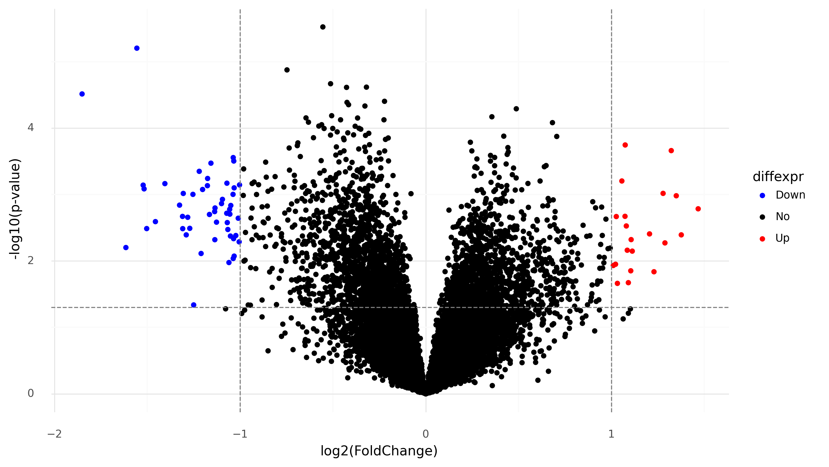
Differentially-expressed genes in bipolar patients during manic phase versus controls.
Larger queries
To query large amounts of data, the API has a pagination system which uses the limit and offset parameters. To avoid overloading the server, calls are limited to a maximum of 100 entries, so the offset allows you to get the next batch of entries in the next call(s).
To simplify the process of accessing all available data, gemmapy includes the
get_all_pages() function which can use the output
from one page to make all the follow up requests
>>> api.get_all_pages(api.get_platforms).head()
   platform_ID platform_short_name  ... taxon_database_name taxon_database_ID
0            1               GPL96  ...                hg38              87.0
1            2             GPL1355  ...                 rn6              86.0
2            3             GPL1261  ...                mm10              81.0
3            4              GPL570  ...                hg38              87.0
4            5               GPL81  ...                mm10              81.0
[5 rows x 13 columns]
Alternative way to access all pages is to do so manually. To see how many available results are there, you can look at the attributes component of the output objects where additional information from the API response is appended.
>>> platform_count = api.get_platforms().attributes['total_elements']
637
After which you can use offset to access all available platforms.
>>> all_platforms = []
>>> for i in range(0,platform_count,100):
...    all_platforms.append(api.get_platforms(offset = i, limit = 100))
>>> pd.concat(all_platforms)
    platform_ID  platform_short_name  ... taxon_database_name taxon_database_ID
0             1                GPL96  ...                hg38              87.0
1             2              GPL1355  ...                 rn6              86.0
2             3              GPL1261  ...                mm10              81.0
3             4               GPL570  ...                hg38              87.0
4             5                GPL81  ...                mm10              81.0
..          ...                  ...  ...                 ...               ...
32         1327             GPL11044  ...                mm10              81.0
33         1328              GPL7182  ...                hg38              87.0
34         1330             GPL33408  ...                 rn6              86.0
35         1331             GPL32159  ...                mm10              81.0
36         1332  014850_4x44K_Merged  ...                hg38              87.0
[637 rows x 13 columns]
Many endpoints only support a single identifier:
>>> api.get_dataset_annotations(["GSE35974","GSE12649"])
...Error Traceback...
In these cases, you will have to loop over all the identifiers you wish to query and send separate requests:
>>> annots = {}
>>> for dataset in ["GSE35974","GSE12649"]:
...   annots[dataset] = api.get_dataset_annotations(dataset)
>>> annots
{'GSE35974':        class_name  ...   object_class
 0  biological sex  ...    BioMaterial
 1         disease  ...    FactorValue
 2         disease  ...    FactorValue
 3  biological sex  ...    BioMaterial
 4       labelling  ...    BioMaterial
 5         disease  ...    FactorValue
 6   organism part  ...  ExperimentTag
 [7 rows x 5 columns],
 'GSE12649':       class_name  ...   object_class
 0        disease  ...    FactorValue
 1      labelling  ...    BioMaterial
 2        disease  ...    FactorValue
 3  organism part  ...  ExperimentTag
 [4 rows x 5 columns]}
Raw endpoints
The previous version of gemmapy exposed raw API endpoints directly while this
version processes the api output into pandas DataFrames for most cases. The old
raw outputs are still accessible however under the raw component of the
GemmaPy instance. In general these functions take the same arguments (with the exception
of taxa and uris arguments for anything that accepts a filter and result_sets argument
of get_result_sets())
>>> api.raw.get_datasets_by_ids([1])
{'data': [{'accession': 'GSE2018',
           'batch_confound': None,
           'batch_effect': 'NO_BATCH_EFFECT_SUCCESS',
           'batch_effect_statistics': 'This data set may have a batch artifact '
                                      '(PC 2), p=0.69477',
           'bio_assay_count': 34,
           'curation_note': None,
           'description': 'Bronchoalveolar lavage samples collected from lung '
                          'transplant recipients.  Numeric portion of sample '
                          'name is an arbitrary patient ID and AxBx number '
                          'indicates the perivascular (A) and bronchiolar (B) '
                          'scores from biopsies collected on the same day as '
                          'the BAL fluid was collected.  Several patients have '
                          'more than one sample in this series and can be '
                          'determined by patient number followed by a lower '
                          'case letter.  Acute rejection state is determined '
                          'by the combined A and B score - specifically, a '
                          'combined AB score of 2 or greater is considered an '
                          'acute rejection.',
           'external_database': 'GEO',
           'external_database_uri': 'http://www.ncbi.nlm.nih.gov/geo/',
           'external_uri': 'https://www.ncbi.nlm.nih.gov/geo/query/acc.cgi?acc=GSE2018',
           'geeq': {'batch_corrected': False,
                    'corr_mat_issues': '2',
                    'id': 557,
                    'no_vectors': False,
                    'public_quality_score': 0.9976340682316643,
                    'public_suitability_score': 0.875,
                    'q_score_batch_info': 1.0,
                    'q_score_outliers': 1.0,
                    'q_score_platforms_tech': 1.0,
                    'q_score_public_batch_confound': 1.0,
                    'q_score_public_batch_effect': 1.0,
                    'q_score_replicates': 1.0,
                    'q_score_sample_correlation_variance': 3.716509481654169e-05,
                    'q_score_sample_mean_correlation': 0.9822784200037354,
                    'q_score_sample_median_correlation': 0.9834384776216498,
                    'replicates_issues': '0',
                    's_score_avg_platform_popularity': 1.0,
                    's_score_avg_platform_size': 0.0,
                    's_score_missing_values': 1.0,
                    's_score_platform_amount': 1.0,
                    's_score_platform_tech_multi': 1.0,
                    's_score_publication': 1.0,
                    's_score_raw_data': 1.0,
                    's_score_sample_size': 1.0},
           'id': 1,
           'last_needs_attention_event': {'_date': datetime.datetime(2018, 10, 2, 20, 57, 53, tzinfo=tzutc()),
                                          'action': 'U',
                                          'action_name': 'Update',
                                          'detail': None,
                                          'event_type_name': 'DoesNotNeedAttentionEvent',
                                          'id': 25176178,
                                          'note': 'Does not need attention.',
                                          'performer': 'amansharma'},
           'last_note_update_event': None,
           'last_troubled_event': None,
           'last_updated': datetime.datetime(2024, 2, 10, 8, 31, 41, 417000, tzinfo=tzutc()),
           'metadata': None,
           'name': 'Human Lung Transplant - BAL',
           'needs_attention': False,
           'number_of_array_designs': 1,
           'number_of_bio_assays': 34,
           'number_of_processed_expression_vectors': 22283,
           'short_name': 'GSE2018',
           'source': '',
           'taxon': {'common_name': 'human',
                     'external_database': {'description': 'Genome Reference '
                                                          'Consortium Human '
                                                          'GRCh38.p13 '
                                                          '(GCA_000001405.28)',
                                           'external_databases': [{'description': None,
                                                                   'external_databases': [],
                                                                   'id': 94,
                                                                   'last_updated': datetime.datetime(2022, 6, 30, 7, 0, tzinfo=tzutc()),
                                                                   'name': 'hg38 '
                                                                           'annotations',
                                                                   'release_url': 'https://www.ncbi.nlm.nih.gov/datasets/genome/GCA_000001405.28/',
                                                                   'release_version': 'GRCh38.p13',
                                                                   'uri': 'https://hgdownload.cse.ucsc.edu/goldenpath/hg38/database/'},
                                                                  {'description': 'Annotations '
                                                                                  'provided '
                                                                                  'by '
                                                                                  'NCBI '
                                                                                  'Genome '
                                                                                  'and '
                                                                                  'used '
                                                                                  'by '
                                                                                  'the '
                                                                                  'RNA-Seq '
                                                                                  'pipeline '
                                                                                  'for '
                                                                                  'human '
                                                                                  'data.',
                                                                   'external_databases': [],
                                                                   'id': 124,
                                                                   'last_updated': datetime.datetime(2023, 1, 17, 20, 27, 55, 59000, tzinfo=tzutc()),
                                                                   'name': 'hg38 '
                                                                           'RNA-Seq '
                                                                           'annotations',
                                                                   'release_url': 'https://ftp.ncbi.nlm.nih.gov/genomes/all/annotation_releases/9606/110/',
                                                                   'release_version': '110',
                                                                   'uri': 'https://www.ncbi.nlm.nih.gov/datasets/genome/GCF_000001405.40/'}],
                                           'id': 87,
                                           'last_updated': datetime.datetime(2022, 6, 30, 7, 0, tzinfo=tzutc()),
                                           'name': 'hg38',
                                           'release_url': 'https://www.ncbi.nlm.nih.gov/datasets/genome/GCA_000001405.28/',
                                           'release_version': 'GRCh38.p13',
                                           'uri': 'https://genome.ucsc.edu/cgi-bin/hgTracks?db=hg38'},
                     'id': 1,
                     'ncbi_id': 9606,
                     'scientific_name': 'Homo sapiens'},
           'taxon_id': 1,
           'technology_type': None,
           'trouble_details': 'No trouble details provided.',
           'troubled': False}],
 'filter': 'id = 1',
 'group_by': ['id'],
 'limit': 20,
 'offset': 0,
 'sort': {'direction': '+', 'order_by': 'id'},
 'total_elements': 1}